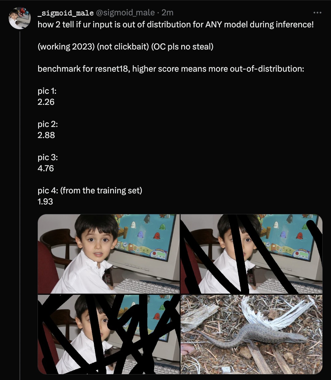
how 2 tell if ur input is out of distribution given only model weights

[dkirmani]

(Hastily-written code to reproduce these findings is available here. It also contains some extraneous logic.)

[Dan H]

There’s a literature on this topic. (paper list, lecture/​slides/​homework)

[dkirmani]

I resent the implication that I need to “read the literature” or “do my homework” before I can meaningfully contribute to a problem of this sort.

The title of my post is “how 2 tell if ur input is out of distribution given only model weights”. That is, given just the model, how can you tell which inputs the model “expects” more? I don’t think any of the resources you refer to are particularly helpful there.

Your paper list consists of six arXiv papers (1, 2, 3, 4, 5, 6).

Paper 1 requires you to bring a dataset.

We propose leveraging [diverse image and text] data to improve deep anomaly detection by training anomaly detectors against an auxiliary dataset of outliers, an approach we call Outlier Exposure (OE). This enables anomaly detectors to generalize and detect unseen anomalies.

Paper 2 just says “softmax classifers tend to make more certain predictions on in-distribution inputs”. I should certainly hope so. (Of course, not every model is a softmax classifer.)

We present a simple baseline that utilizes probabilities from softmax distributions. Correctly classified examples tend to have greater maximum softmax probabilities than erroneously classified and out-of-distribution examples, allowing for their detection.

Paper 3 requires you to know the training set, and also it only works on models that happen to be softmax classifiers.

Paper 4 requires a dataset of in-distribution data, it requires you to train a classifier for every model you want to use their methods with, and it looks like it requires the data to be separated into various classes.

Paper 5 is basically the same as Paper 2, except it says “logits” instead of “probabilities”, and includes more benchmarks.

We [...] find that a surprisingly simple detector based on the maximum logit outperforms prior methods in all the large-scale multi-class, multi-label, and segmentation tasks.

Paper 6 only works for classifiers and it also requires you to provide an in-distribution dataset.

We obtain the class conditional Gaussian distributions with respect to (low- and upper-level) features of the deep models under Gaussian discriminant analysis, which result in a confidence score based on the Mahalanobis distance.

It seems that all of the six methods you referred me to either (1) require you to bring a dataset, or (2) reduce to “Hey guys, classifiers make less confident predictions OOD!”. Therefore, I feel perfectly fine about failing to acknowledge the extant academic literature here.

(Additionally, the methods in my post were also replicated in language models by @voooooogel:

)

[Chris_Leong]

I’m slightly confused here by the results here. Is there idea that pictures with texta drawn over them are out of distribution?

If so, should I be more impressed by the difference between pic 1 and pic 2? It doesn’t seem to be that much, although it’s hard to tell from just seeing the metric from 4 images.

I’m also somewhat confused about why this works. It seems to me that within a distribution it’s perfectly fine to have some areas where it changes quickly and some where it changes slowly. And it seems like this would break this metric. I assume there’s something obvious that I’m missing.

[dkirmani]

I’m also somewhat confused about why this works

Abstraction is about what information you throw away. For a ReLU activation function, all negative inputs are mapped to zero—you lose information there, in a way that you don’t when applying a linear transformation.

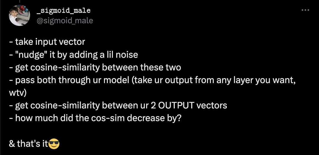
Imagine your model (or a submodule thereof) as a mapping from one vector space to another. In order to focus on the features relevant to the questions you care about (is the image a truck, is it a lizard, …) you throw away information that is not relevant to these questions—you give it less real-estate in your representation-space. We can expect more out-of-distribution regions of input-space to be “pinched” by the model—they’re not represented as expressively as are the more in-distribution regions of input-space.

So if your cosine-similarity decreases less when you nudge your input, you’re in a more “pinched” region of input-space, and if it decreases more, you’re in a more “expanded” region of input space—which means the model was tuned to focus on that region, which means it’s more in-distribution.

[Chris_Leong]

Ok, that’s fascinating! Thanks for the explanation.

[dkirmani]

Is there idea that pictures with texta drawn over them are out of distribution?

Yes, the idea is that images that have been taken with a camera were present in the training set, whereas images that were taken with a camera and then scribbled on in GIMP were not.

If you refer to section 4.2 in the paper that leogao linked, those authors also use “corrupted input detection” to benchmark their method. You’re also welcome to try it on your own images—to run the code you just have to install the pip dependencies and then use paths to your own files. (If you uncomment the block at the bottom, you can run it off your webcam in real-time!)

[leogao]

Sounds very closely related to gradient based OOD detection methods; see https://​​arxiv.org/​​abs/​​2008.08030

[dkirmani]

We introduced the concept of the space of models in terms of optimization and motivated the utility of gradients as a distance measure in the space of model that corresponds to the required amount of adjustment to model parameters to properly represent given inputs.

Looks kinda similar, I guess. But their methods require you to know what the labels are, they require you to do backprop, they require you to know the loss function of your model, and it looks like their methods wouldn’t work on arbitrarily-specified submodules of a given model, only the model as a whole.

The approach in my post is dirt-cheap, straightforward, and it Just Works™. In my experiments (as you can see in the code) I draw my “output” from the third-last convolutional state. Why? Because it doesn’t matter—grab inscrutable vectors from the middle of the model, and it still works as you’d expect it to.

[Gerald Monroe]

You could also train an autoencoder on the training set and then autoencode the input image and measure the residual part.

[dkirmani]

Yep, but:

given only model weights

Also, the cossim-based approach should work on arbitrary submodules of a given model! Also it’s fast!