tl;dr: We compute the evolution of the local learning coefficient (LLC), a proxy for model complexity, for an algorithmic transformer. The LLC decreases as the model learns more structured solutions, such as head specialization.

This post is structured in three main parts, (1) a summary, giving an overview of the main results, (2) the Fine Print, that delves into various cross-checks and details and (3) Discussion and Conclusions.

Structure Formation in Algorithmic Transformers

In this work we study the development of simple algorithmic transformers, which are transformers that learn to perform algorithmic tasks. A major advantage of this setup is that we can control several (hyper)parameters, such as the complexity of the training data and network architecture. This allows us to do targeted experiments studying the impacts of these parameters on the learning dynamics. The main tool we use to study the development is the Local Learning Coefficient (LLC) and we choose cases where we have a reverse-engineered solution.

Why use the LLC for this purpose? It is a theoretically well motivated measure of model complexity defined by Lau et.al. For an overview of Singular Learning Theory (which serves as the theoretical foundation for the LLC) see Liam Carol’s Distilling SLT sequence. For a brief overview of the LLC see e.g. this post.

We use the same setup as CallumMcDougall’s October Monthly Algorithmic Mech-Interp Challenge. The model is an attention only transformer, trained on sorting numbers with layer norm and weight decay on a cross-entropy loss function using the Adam optimizer. The residual stream size is 96 and the head dimension is 48. It is trained on sequences of the form

[14, 47, 15, 6, 27, 41, 8, 16, 4, 48, SEP, 4, 6, 8, 14, 15, 16, 27, 41, 47, 48]

and to predict the next token starting at the separation token. The numbers in the list are sampled uniformly from 0 to 50, which together with the separation token produce a vocabulary of 52 tokens. Numbers do not repeat in the list. The images making up the gifs can be found here.

1-Head Model

Let’s first look at the case of a 1-head transformer:

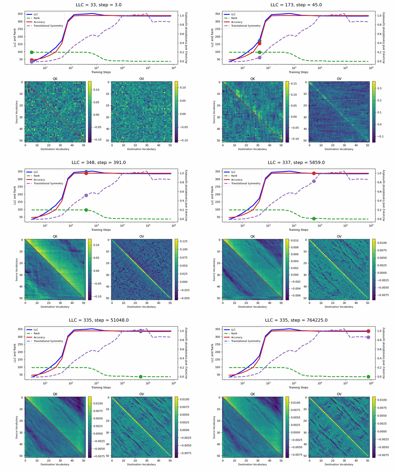
**Structure formation for 1-head attention model sorting lists.** The heat-maps show the full QK and OV circuits. The upper plot shows the LLC together with other measures such as the translational symmetry^[1] and the Rank, which is defined as the sum of the matrix ranks of the heat maps.

The model reaches 100% accuracy around training step 100, confirming that a single attention head is sufficient for sorting, as noted in previous work. Once maximum accuracy is reached, the full QK and OV circuits^[2] behave as described by Callum for the 2-head model:

In the QK circuit, source tokens attend more to the smallest token in the list larger than themselves. This results in a higher value band above the diagonal and a lower value band below the diagonal.
The OV circuit copies tokens, as seen by the clear positive diagonal pattern.

In addition, we observe a transition around training step 1000, where the LLC decreases while the accuracy stays unchanged. This is supported by a drop in the sum of the ranks^[3] of the matrices in the heat maps.

It also coincides with the formation of the off-diagonal stripes in the OV-circuit. We speculate that these are simpler than the noisier off-diagonal OV pattern observed at peak LLC, and correspond to the translational symmetry of the problem. We define a Translational Symmetry measure^[1] (see purple line in the plot) to capture the degree to which the circuits obey this symmetry. It increases throughout most of the training, even after the other measures stabilize.

2-Head Model

Let’s now turn our attention to the 2-head transformer in Callum’s original setup.

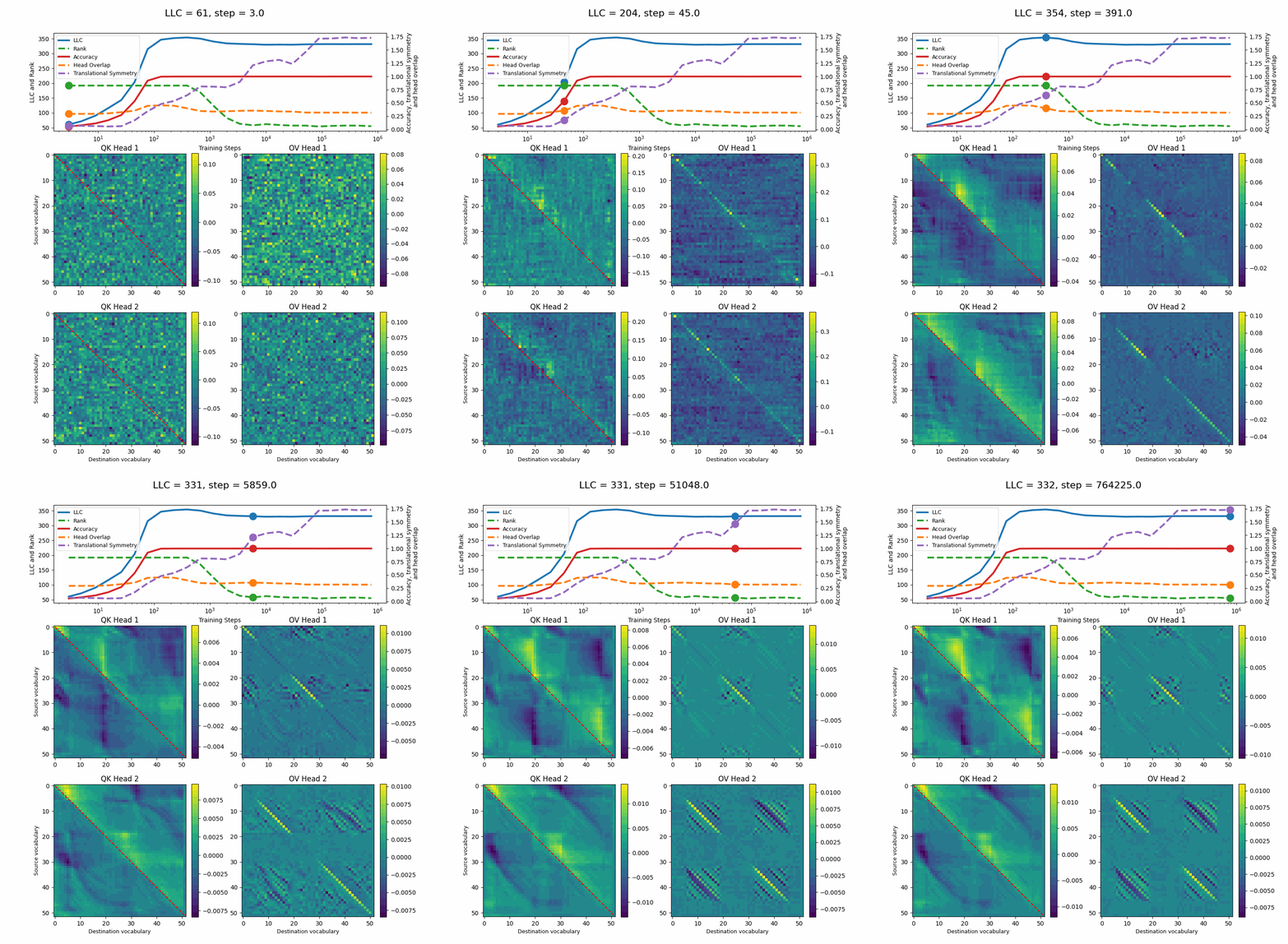
**Structure formation for 2-head attention model sorting lists.** The heat-maps show the full QK and OV circuits. The upper plot shows the LLC together with other measures such as the translational symmetry^[1], the head overlap^[4] and the Rank, which is defined as the sum of the matrix ranks of the heat maps.

We see a lot of qualitative similarities to the evolution of the full QK and OV circuits for the 1-head model. As the LLC begins to drop (around training step 1000), we note the following:

QK circuit: Slight changes^[5] to the attention pattern, which crystallize into triangular regions late in the training, long after the LLC has stabilized.
OV circuit: The heads specialize, splitting the vocabulary between them in contiguous, almost periodic, regions.

The specialization in the OV circuits of the heads can be interpreted as a simpler solution compared to the model at peak LLC, as each head attends to less vocabulary. This is reinforced by the drop in the Rank. In addition, we also introduce a measure of the overlap^[4] between the two heads. The overlap is maximal at peak LLC and decreases with it. The translational symmetry measure increases step-wise during training and remains in-flux after the other measures stabilize.

In summary, we find that the LLC correctly captures the relevant developmental stages that a simple algorithmic transformer undergoes in learning how to sort lists. We can identify how the learned solution simplifies, as the LLC drops at the same time as the emergence of additional structure in the OV circuit, such as head specialization. It seems intuitive to interpret the LLC drop to be due to this specialization, but we don’t have conclusive evidence for this.

The Fine Print

For more details and caveats, keep on reading!

In this section we discuss several variations of the setup discussed above, to study the robustness of head specialization. We experiment with removing layer norm and weight decay, with adding more heads and with making changes to the training data such as changing the size of the vocabulary, changing the length of the lists and perturbing the training data.

2-Head Model: Re-loaded

Removing Layer Norm

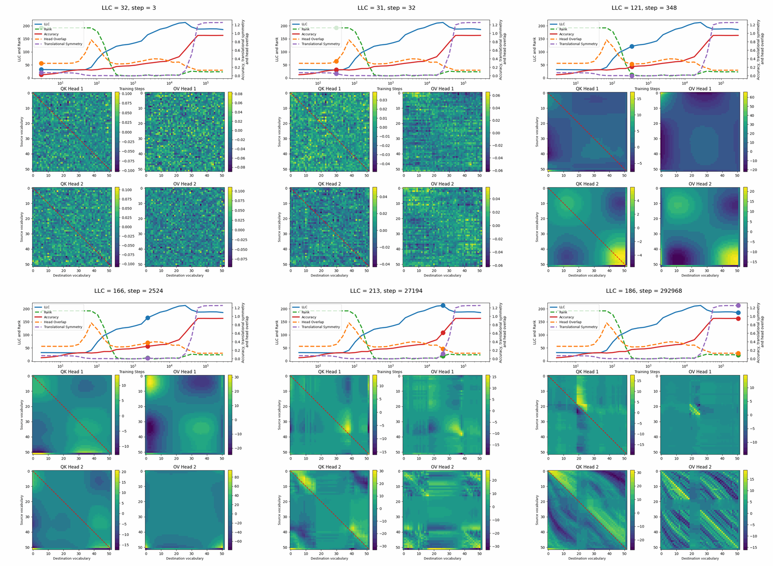
Removing Layer Norm leads to a protracted learning curve and a model that learns to sort with around 90% accuracy after 60k training steps. Notably, the LLC peaks earlier, after 27k steps. It begins to decrease immediately after the peak, up until 60k steps, which coincides with full QK and OV circuits developing some similar patterns to the 2-head baseline model with layer norm. This is captured by the translational symmetry increasing significantly and the head overlap decreasing^[6] as the heads specialize.

The sum of the ranks of the matrices in the heat maps on the other hand, decreases steeply around training step 100. At this point, the heat maps develop into a dipole-like pattern, which look quite a lot less noisy than a random matrix or even the learned solution in the end of the training. Unfortunately, despite the simplicity of the matrices, the model cannot sort at this stage. As the LLC peaks, the Rank increases very slightly, reflecting the new learned solution. Thus, the ranks of the OV and QK circuits as a proxy for model complexity should be considered and interpreted with care, as they don’t always detect relevant transitions in the model.

Removing Weight Decay

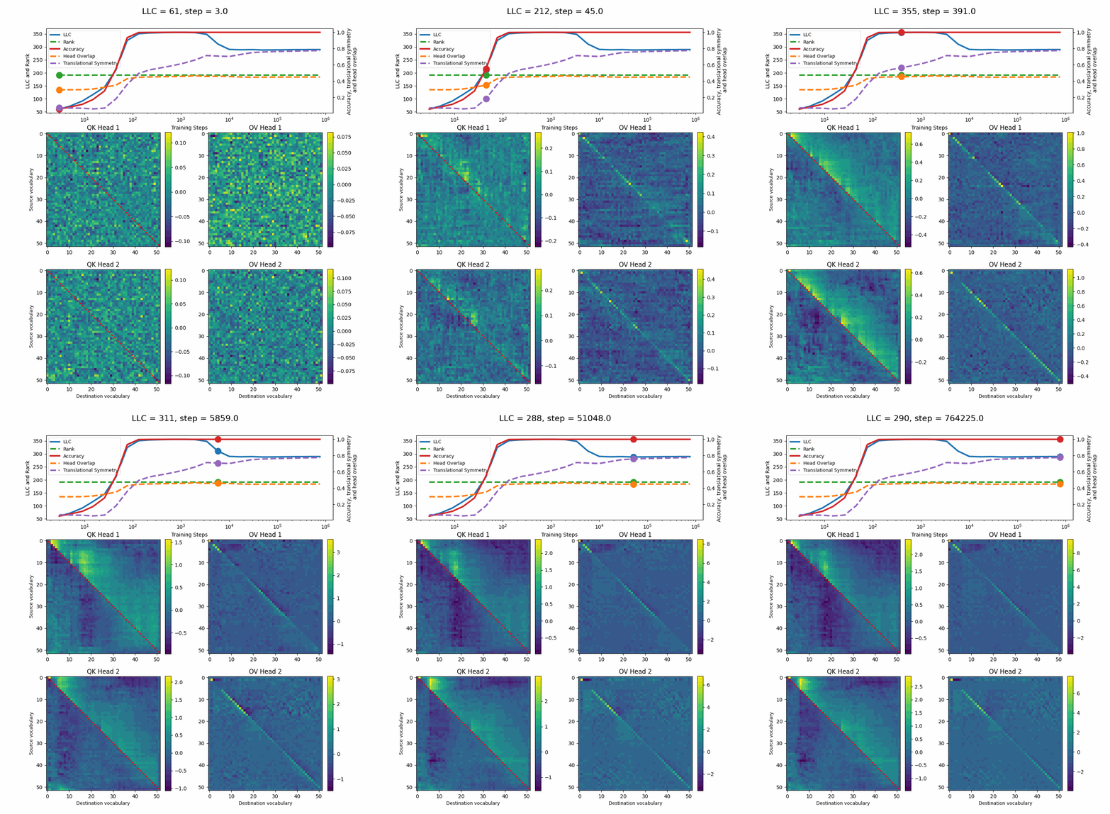
Removing Weight Decay leads to a less clean structure in the QK and OV circuits. We still recognize some familiar patterns from the baseline 2-head model. The translational symmetry increases during most of the training, but it peaks at around 0.8, quite a lot below the maximal values for the baseline 2-head model (~1.75) and for the 2-head model without Layer Norm (~1.25) discussed above. The overlap between the heads is also larger compared to previous models, and it has a very small bump, which decreases with the LLC. The Rank doesn’t capture any of the changes in the model, remaining constant during the entire training.

The decrease in LLC coincides with the QK circuits developing a distinct positive region in the top left corner of the diagonal (which we don’t quite understand) and the OV circuit specializing to attend to different vocabulary regions. Unlike in the 2-head baseline model, there is no further crystallization of the structure later in the training. The changes we do observe as the LLC decreases, are not well captured by any of the other measures.

Removing both Layer Norm and Weight Decay

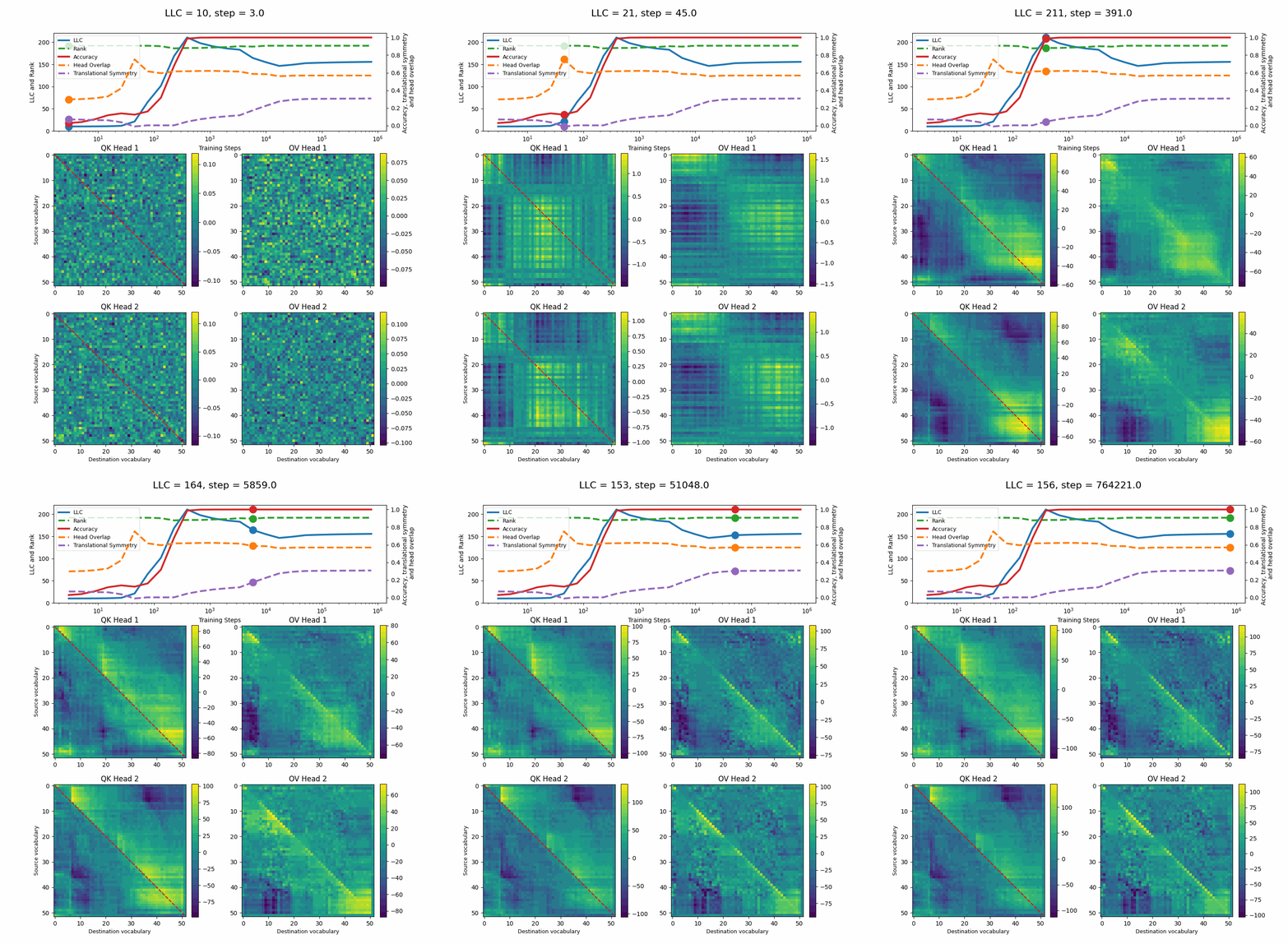
**Removing Weight Decay and Layer Norm** leads to weaker specialization, no significant Rank drop and no clear crystallization of the OV circuits late in the training. The LLC mirrors the translational symmetry, and flatlines once the circuits are stable.

Removing both Layer Norm and Weight Decay^[7] leads to a model that can sort with 100% accuracy^[8], but implements a significantly noisier solution.

The LLC peaks shortly before step 400 and decreases slowly until step 10k, after which it starts increasing slightly until the end of training. During the intermediate phase when the LLC decreases, the full QK and OV circuits develop more structured patterns, similar to the 2-head baseline model. The translational symmetry increases during this stage, but its maximal value (~0.35) is quite smaller than for the other models. The head overlap decreases slightly with the LLC and is larger than for all previous models (~0.6).

Here too, the LLC decrease happens during the training steps when the OV circuits specialize for each head and the QK circuits develop a more distinctly positive region above the diagonal. The new measures we introduce, the translational symmetry and the head overlap, manage to capture these changes as well. The Rank is constant throughout training.

Adding Noise

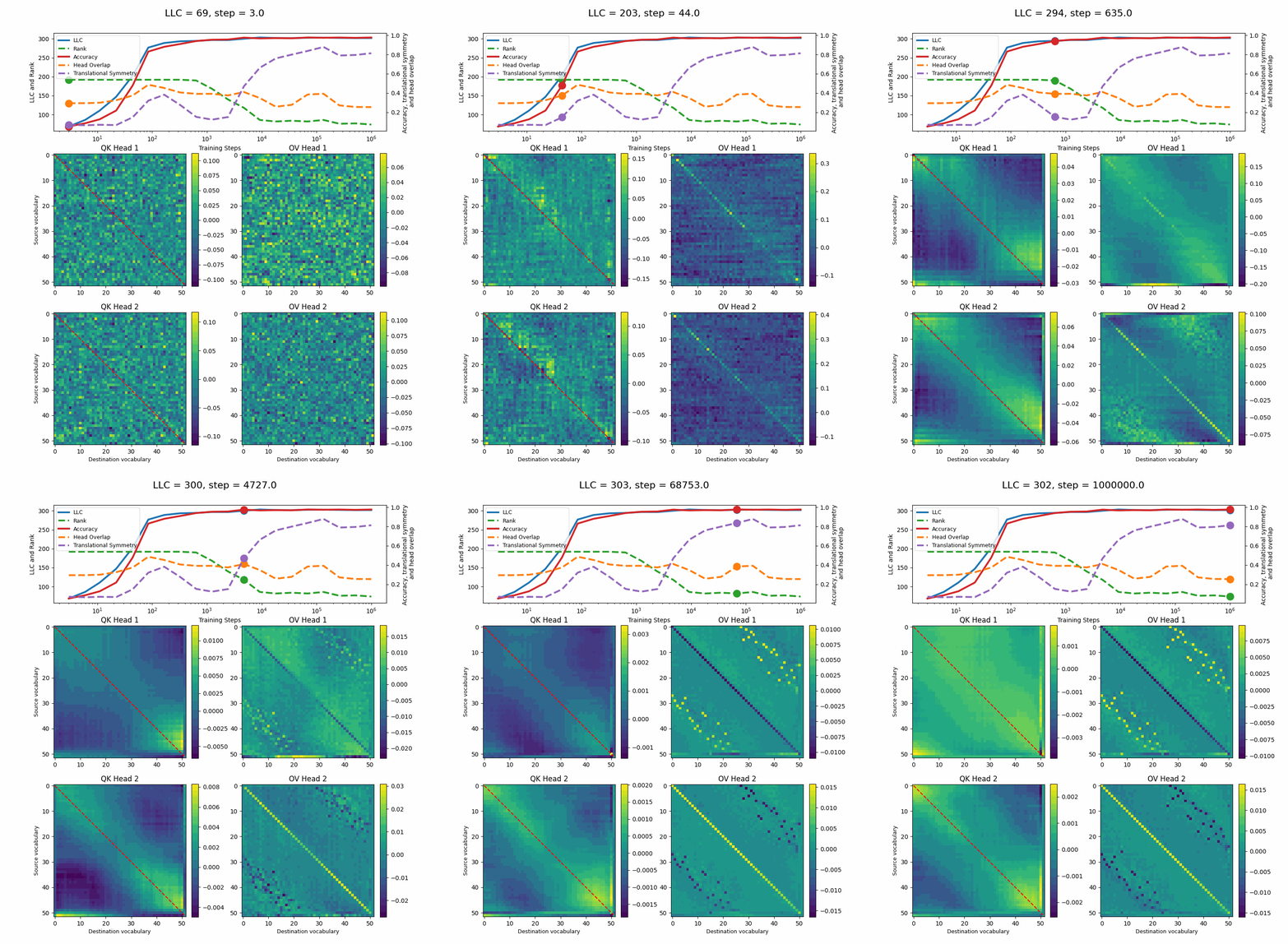
If you add noise^[9] to the training data, there is no drop in the LLC and the OV circuits of the heads don’t specialize to split vocabulary regions. The full OV circuit of head 2 develops several of the features of the original solution, while the OV circuit for head 1 seems to settle into the role of an “anti-state” to head 2. We will rediscover this phenomenon when discussing architectures with 3 and 4 heads below. The QK circuits do not behave at all like the baseline 2-head model, and we don’t understand why.

Despite the missing head specialization, the OV circuits develop a clear diagonal pattern. The transition to the “state”-”anti-state” setup for both heads, is capture by a drop in the sum of the matrix ranks and an increase in the translational symmetry measure, after 2.4k training steps. This is not reflected in the LLC curve, and could be due to the fact that the Rank and the translational symmetry treat the full OV and QK circuits as independent, when they in fact are not.

The accuracy for this model has been computed on a non-noisy validation set.

**Adding noise to the training data** leads to a state/anti-state specialization, where head 1 settles into a state opposite to head 2. Unlike in all the other cases, the LLC does not drop.

Number of vocabulary regions

A key feature of the solution the model learns, is the separation of the vocabulary in the OV circuits, as the heads specialize. We wanted to know what drives the number of regions. To that end we tried changing the size of the vocabulary and the size of the lists we are sorting.

Here is the 2-head model, trained on sorting lists with a vocabulary size of 202 (instead of 52):

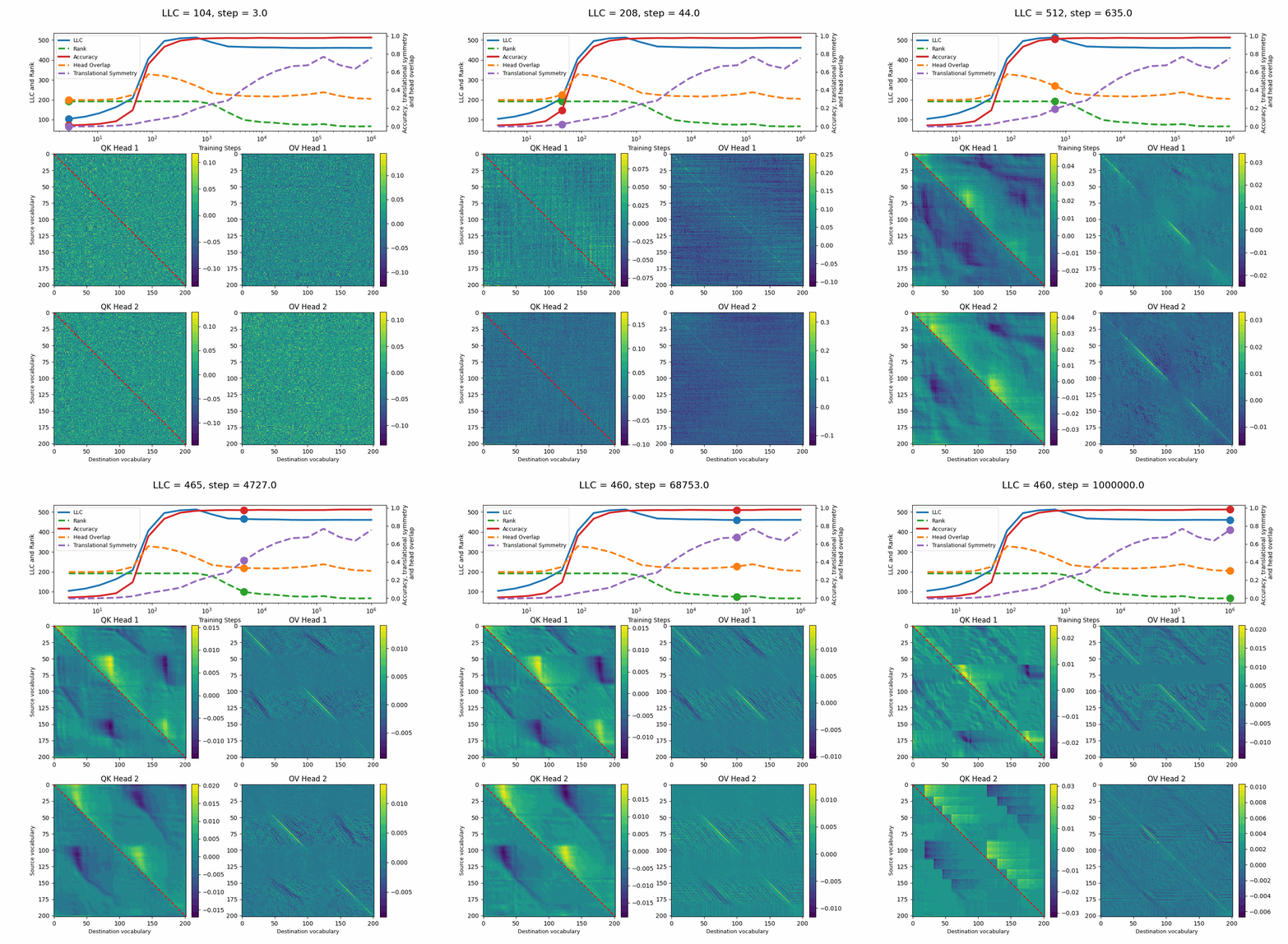
**Increasing vocabulary size to 202** leads to similar dynamics as the base-line model with a vocabulary size of 52. The number of regions remains unchanged, the size of the regions increases.

The number of regions remains the same, they grow larger instead of separating further.

Increasing the length of the list increases the number of regions. Here is the 2-head model, trained on sorting lists with length 20 (instead of 10) and vocabulary size of 52 (as the baseline model):

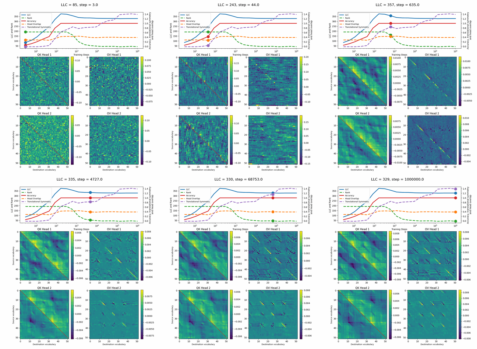
**Increasing list length to 20** leads to similar dynamics as the base-line model with a list length of 10. The number of regions increases, to form a larger number of smaller regions with a periodic structure.

Here the LLC diagnostics works fairly similar to the 2-head baseline model, with the QK and OV patterns zooming out to show more regions.

Adding More Heads

We observe that the 2 heads in a transformer model with a single layer, specialize into handling different regions of the vocabulary. A natural follow up question to ask, is if the specializing trend continues when adding more heads in the same layer. Does each head get a region or two of the vocabulary? Not really.

**Increasing number of heads to 3** leads to head 1 and 2 specializing like in the base-line 2-head model. The 3rd head settles into an anti-state, (approximately) proportional to the sum of the OV circuits of the other heads.

During peak LLC, the 3-head model does in fact divide the vocabulary in between the 3 heads, with the 3rd head handling a smaller vocabulary range than the other heads. As the LLC drops, this vocabulary range is taken over by the 2nd head, leaving the 1st and 2nd heads to operate very similarly to the baseline 2-head model. Meanwhile, the 3rd head settles into an “anti-state” head, with its OV circuit (approximately) negatively proportional to the sum of the OV circuits of the other two heads.

Adding a 4th head, leads to heads 1 and 4 specializing and splitting the dictionary between them, similarly to the baseline 2-head model. Head 2 settles into the “anti-state” we discussed previously; it initially covers a small vocabulary range, and then settles into a negative. This happens around training step 5000, at the same time as a sharp drop in the LLC. Head 3, on the other side, has a significant overlap with head 4 for much of the training, before it settles into a state very similar to the sorting solution of the 1-head model around step 100k. The LLC drops slightly as this happens.

After this, the LLC and the full OV and QK circuits seem stable.

**Increasing number of heads to 4** leads to head 1 and 4 specializing like in the base-line 2-head model. The 2nd head settles into an anti-state, (approximately) proportional to the sum of the OV circuits of the other heads, whereas the 3rd head settles into a state similar to the OV circuit of the 1-headed model. The LLC decreases captures these specializations.

Other algorithmic transformers

We also considered the cumulative sum algorithmic transformer from Callum’s monthly challenges. We found that this transformer had a much simpler evolution, where the LLC simply goes up and plateaus as the accuracy reaches 100%. Looking at the circuits, we also don’t find a simplification, but rather that the model goes directly to the final structure.

Related work

Developmental stages have been studied by Hoogland et. al. (2024) within the context of SLT, where the authors also find that a drop in the LLC corresponds to simplification when training a transformer on linear regression. Using another approach, Chen et.al. (2024) identified developmental stages when studying Syntactic Attention Structure in BERT. The LLC evolution of neural networks trained on the algorithmic task of modular addition has previously been studied by Panickssery and Vaintrob (2023) in the context of grokking.

Discussion and Conclusions

We employed the Local Learning Coefficient (LLC) as a diagnostic tool for tracking the development of complexity in transformers trained on a couple simple algorithmic tasks. We found that the list sorting model has a fairly rich evolution.

Specifically, in the baseline model with 2-heads, we observed:

head-specialization, as the LLC decreases.
crystallization of the positive regions above the diagonal in the QK circuits and of the periodic regions in the OV circuits later on in the training (long after the LLC decrease).

We interpret head specialization, where the OV circuits of each head handles unique parts of the vocabulary, as a simpler solution than the OV circuits of both heads attending to the entire available vocabulary (as is the case at peak LLC). The head overlap measure was intended to capture this specialization. In the variations of the baseline setup we observe that:

If we have only 1 head, there is no specialization, but we still notice a (somewhat weaker) drop in the LLC, which coincides with the sum of the matrix ranks decreasing. This could be interpreted as a simpler, less noisy solution. However, it doesn’t immediately fit well with the rest of our interpretations.
The specialization is still present after removing layer norm, weight decay, or both, but the QK and OV circuits are significantly noisier. In these cases, the sum of the matrix rank stops being a good measure of the relevant dynamics.
The head specialization, in the sense of the heads splitting the vocabulary, is not present if training with perturbed data. We do get a different kind of specialization in the OV circuits, into a “state”-”anti-state” head setup. This is not captured by the LLC.
The size of the LLC drop is not proportional to the head-specialization in the full OV circuits, or the formation of the expected regions in the QK circuits.

It is more difficult to judge the phenomenon of crystallization, as defined above. It is not clearly present in the models without layer norm and/or weight decay, and it’s unclear what role it plays in the model. In the baseline 2-head model, we can cleanly separate between the beginning of head specialization and the crystallization later in the training. The latter is captured by the translational symmetry measure, but not the LLC.

In general, we note that the more established measure (matrix rank) and the new^[10] measures (translational symmetry, head overlap) we introduce here have their weaknesses. In particular, they all treat the OV and QK circuits as independent, which they are not. A major advantage of the LLC is that it doesn’t require specific knowledge of the ground truth of the model or any additional specifics of the setup to compute.

Statement of Contributions: Einar ran all of the experiments, analyzed and interpreted the results, and produced the figures. Jasmina contributed to analyzing and interpreting the results. The authors wrote the post together.

Acknowledgements: Einar’s research was supported by the ERA Fellowship. He would like to thank the ERA fellowship for its financial and intellectual support. Jasmina’s research was supported by an LTFF grant. She thanks the ERA Fellowship for kindly providing office space. The authors also thank Jesse Hoogland and Rudolf Laine for mentorship and valuable input during the research. A big thanks to Dan Murfet, Jesse Hoogland, Stefan Heimersheim and Nicky Pochinkov for valuable feedback on the post.

^
This measure is meant to capture the degree to which the circuits reflect the (approximate) translational symmetry of the vocabulary: Away from the vocabulary edges, the circuits should be translation invariant in the sense that the attention pattern should only depend on the difference between two numbers, not on their magnitude. This is expected to translate into patterns that are uniform along lines parallel to the diagonal. To capture this, we look at the irregularity perpendicular to the diagonal, minus the irregularity parallel to the diagonal, where we by irregularity mean the difference between an element and the average of its neighbors. We find that this measure roughly captures the stripe-like pattern that can be seen in the figures.
$\frac{\sum_{i j} | W_{i, j} - \frac{W_{i - 1, j + 1} + W_{i + 1, j - 1}}{2} | - | W_{i, j} - \frac{W_{i - 1, j - 1} + W_{i + 1, j + 1}}{2} |}{¯ ¯¯¯¯ ¯ W \sum_{i j}}$
The sum is taken over all $i$ and $j$ except the ones closest to the edge of the matrix.
^
The full QK circuit is defined as
$W_{E} W_{Q}^{h} (W_{K}^{h})^{T} W_{E}^{T}$
and the full OV circuit is defined as
$W_{E} W_{V}^{h} W_{O}^{h} W_{U}$
$h$ denotes the attention head. When we say simply OV or QK circuit, we mean the full circuits listed in this footnote.
^
The rank can be interpreted as a general measure of the complexity of a matrix. We use this as an alternative way to estimate the combined complexity of the OV and QK circuits.
^
The head overlap is, as indicated by the name, the overlap between the circuits of two heads. We define the overlap of two circuits as
$O (c^{h_{k}}, c^{h_{ℓ}}) = 1 - \frac{\sum_{i j} ∣ ∣ W_{i j}^{h_{k}} - W_{i j}^{h_{ℓ}} ∣ ∣}{\sum_{i j} ∣ ∣ W_{i j}^{h_{k}} ∣ ∣ + ∣ ∣ W_{i j}^{h_{ℓ}} ∣ ∣}$
where $c^{h_{k}}, c^{h_{ℓ}}$ denote two OV or QK circuits, with matrices $W_{i j}^{h_{k}}, W_{i j}^{h_{ℓ}}$ as displayed in the heatmaps, belonging to heads $k$ and $ℓ$ with $k \neq ℓ$ . For a 2-head model we average the overlap between the OV and QK circuits. If more heads are available, we average over circuits and over all head combinations.
^
compared to other stages of the training
^
Interestingly, the head overlap is smaller for this model, compared to the baseline 2-head case when Layer Norm is active. But on the other hand, most of the vocabulary is handled by head 2.
^
There is still some leftover regularization in our model, hidden in the Adam Optimizer, despite removing Weight Decay.
^
When removing only the Layer Norm, we found that the model reaches at most about 90% accuracy given similar training conditions. We don’t understand why.
^
We did this by iteratively swapping neighbouring elements in the sorted list with probability $40 % / (n_{i + 1} - n_{i})$ , where $n_{i}$ is the value of list element i.
^
We are not claiming that these measures are novel, we simply state that we are not aware of them being established in the AI literature.

Measuring Structure Development in Algorithmic Transformers