Intuitive Explanation of AIXI

[Thomas Larsen]

AIXI is a mathematical notion of an ideal RL agent, developed by Marcus Hutter. The famous formula for AIXI is as follows:

$$a_k={\text{argmax}}_{a_k}\sum _{o_k{r}_k}{\text{max}}_{a_{k+1}}\sum _{o_{k+1}{r}_{k+1}}\dots \sum _{o_m{r}_m}[r_k+\cdots +r_m]\sum _{q:q(a_1\dots a_k)=o_1{r}_1\dots o_m{r}_m}{2}^{-l\left(q\right)}$$

This math seems unintuitive at first (at least to me—why are there so many sums???), and I couldn’t find any simple introductory resources, so this post is my attempt at an intuitive explanation of what this formula means. I try to convey the intuition that AIXI is the obvious formula for an expected reward maximizer in a discrete, finite environment, following the Solomonoff prior.

Setting

AIXI works in the following setting: There is an agent, and an environment, which is a computable function. There is a cartesian boundary between the agent and the environment, meaning that the agent is fully separate from the environment. The agent is uncertain about the environment.

There are a $m$ timesteps, and at each time, each timestep, the agent will perform an action and then receive an observation (a bitstring) and a reward (a number). We will denote the action, reward, and observation taken at the $k$-th timestep as $a_k$, $r_k$, and $o_k$ respectively.

We want our agent to maximize the total reward: $r_1+\cdots +r_m$. We assume that the environment is a program with source code $Q$, which takes as inputs the agents actions and outputs a sequence of observations and reward: $Q(a_1\dots a_k)=o_1{r}_1\dots o_k{r}_k$ .^[1]

Motivating Example

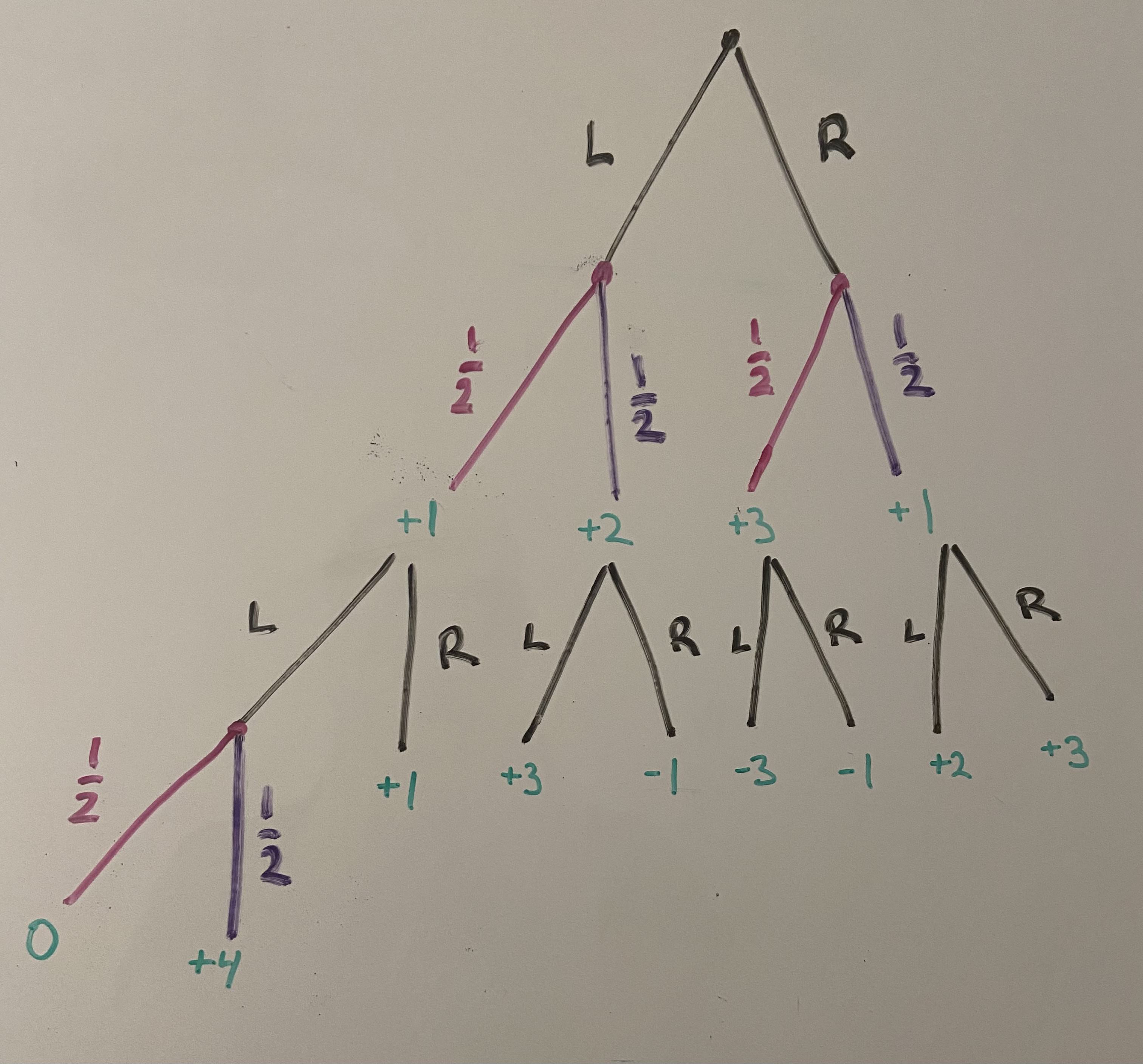
Suppose that we have the following game, where again at each timestep, you can choose between $R$ and $L$. However, this time, you are not sure which world you are in—you have multiple codes that might be running the universe. For example, consider the following game tree:

There are 2 timesteps, and at each timestep you can choose from two actions: L or R. However, in this game you also have uncertainty: after some of your actions, you have uncertainty, represented by the pink and purple branches. We are completely uncertain over each of these splits, and they are independent. At each timestep, you recieve the reward given in green. Think about how you would which action to take first. (You might need to get out pencil and paper!)

.

.

.

Seriously think for at least 5 minutes (by a timer!) about this, or until you get it.

.

.

.

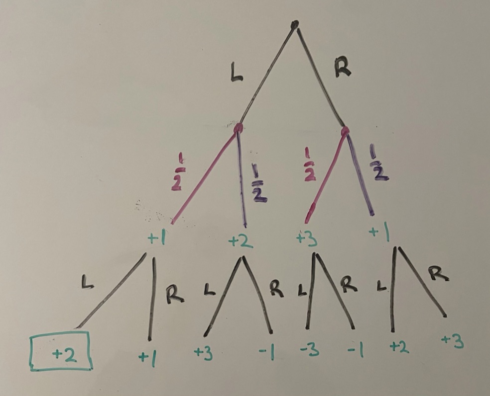
Here’s the most intuitive approach to me: we proceed bottom up, computing how much expected reward there is at each node. The first step is to collapse all of the uncertainty in the last layer. There is only uncertainty in the bottom left node, in this example, and so we simply compute the expectation: $0\left(\frac{1}{2}\right)+4\left(\frac{1}{2}\right)=2$, and replace that node with a $+2$ expected value:

Now, at the bottom of the graph, we are faced with 4 decisions over which action to take. However, it is pretty clear what our agent should do in each of these situations: take the action that maximizes expected reward. So going form the left of the graph to the right, we take L (+2), L (+3), R (-1), and R (+3). Thus, we can add these into the rewards from the first layer.

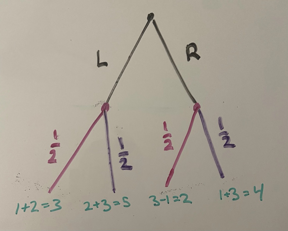
The added values represent total future reward at that point in the game tree. Now, we are back to uncertainty, so we take the expectation at each node:

And thus we see that taking L is better than R, for expected total reward of $+4$. So an ideal agent will choose action L at the first timestep, in this example.

Formalization of 2-step environment

We followed a specific, deterministic procedure, which we can write down into a formula for finding the action that gives us the largest expected reward. The procedure we followed was starting at the bottom later of the graph, and then

1. taking the expectation over rewards.

2. choosing the action with maximum expected future reward.

3. repeating 1-2 for the layer above.

For this example with two actions and two timesteps, writing this in our notation gives: ^[2]

$$a_1={\text{argmax}}_{a_1\in \{L,R\}}\sum _{r_1}P\left(r_1|a_1\right)[r_1+E(r_2|a_1\left)\right]$$

We can evaluate this expectation, which is just the EV of the best action, because we are an ideal agent. That is:

$$E\left(r_2|a_1\right)={\text{max}}_{a_2\in \{L,R\}}\sum _{r_2}P(r_2|r_1,a_1,a_2)r_2$$

Substituting this in yields:

$$a_1={\text{argmax}}_{a_1\in \{L,R\}}\sum _{r_1}P\left(r_1|a_1\right)[r_1+{\text{max}}_{a_2\in \{L,R\}}\sum _{r_2}P(r_2|r_1,a_1,a_2\left)r_2\right]$$

We can rearrange the above expression to something that is more algebraically naturally by moving the $r_1$ inside the second sum, and by realizing that the second action doesn’t effect the first reward, so $P\left(r_1|a_1\right)=P(r_1|a_1,a_2)$. Then we combine the two probabilities to get $P(r_1|a_1,a_2)P(r_2|r_1,a_1,a_2)=P(r_1,r_2|a_1,a_2)$. Substituting this in gives a cleaner algebraic representation of the ideal action:

$$a_1={\text{argmax}}_{a_1\in \{L,R\}}\sum _{r_1}{\text{max}}_{a_2\in \{L,R\}}\sum _{r_2}[r_1+r_2]P(r_1,r_2|a_1,a_2)$$

Generalization to $m$-step environments

Generalizing this to the $k$-th timestep with $m$ total actions is straightforward, we just continue to mix these expectations.

$$a_k={\text{argmax}}_{a_k}\sum _{r_k}{\text{max}}_{a_{k+1}}\sum _{r_{k+1}}\dots {\text{max}}_{a_m}\sum _{r_m}(r_k+\cdots +r_m)P(o_1{r}_1\dots o_m{r}_m|a_1\dots a_m)$$

To see this, start reading the formula from right to left.

• $(r_k+\cdots +r_m)$ gives the future reward conditional on a specific actions $a_1\dots a_m$.

• $P(o_1{r}_1\dots o_m{r}_m|a_1\dots a_m)$ gives the probability of seeing the output $o_1{r}_1\dots o_m{r}_m$ after taking actions $a_1\dots a_m$.

• The term ${\sum }_{r_m}(r_k+\cdots +r_m)P(o_1{r}_1\dots o_m{r}_m|a_1\dots a_m)$ gives the expected future reward, added up over the last times.

• Each sum runs over all of the possible rewards for a given step. The sums correspond to the expectation over the future reward.

• We know that we will take the best action in the future, so we aren’t doing to average over all of the possible actions, we compute based off of the max EV action.

• After this interleaving of sums and max, we are at a node at the very bottom of the tree, which we simply weight by its probability $P(o_1{r}_1\dots o_k{r}_k|a_1\dots a_k)$. The observations here simply refer to which branch of the graph we are in.

One last point: Even though a gave a tree with probabilities in it, the environment here is not stochastic. There is a true program, $q$, that deterministically maps actions to rewards, and our uncertainty comes from just not knowing which $q$ is correct. All of our uncertainty is in the mind.

The Solomonoff Prior

In the previous section, I simply gave you the probabilities that you believed over the possible world. But what if we didn’t know these probabilities? We need a prior that we can then update.

Recall that we modeled the world as some program $Q$. Occam’s razor gives us a natural way to weight the likelihoods of these different programs according to their simplicity. We’ll use length as a measure of simplicity. The Solomonoff prior assigns probability to each program equal to the inverse of the length of the code that outputs them.

$$P(Q=q)=2^{-l\left(q\right)}$$

Here, $l\left(q\right)$ denotes the length of the program $q$. Recall that we defined:

$$P(o_1{r}_1\dots o_k{r}_k|a_1\dots a_k)=P\left(Q\right(a_1\dots a_k)=o_1{r}_1\dots o_k{r}_k)$$

Expanding over the possible programs that could output that sequence gives:

$$P\left(Q\right(a_1\dots a_k)=o_1{r}_1\dots o_k{r}_k)=\sum _{q:q(a_1\dots a_k)=o_1{r}_1\dots o_k{r}_k}P(Q=q)$$$$=\sum _{q:q(a_1\dots a_k)=o_1{r}_1\dots o_k{r}_k}{2}^{-l\left(q\right)}$$

The probability of seeing the output $o_1{r}_1\dots o_k{r}_k$ is equal to all of the different universe source codes $q$, added up according to their probability.

And finally… AIXI

Plugging in the Solomonoff prior into the previous formula gives

$$a_k={\text{argmax}}_{a_k}\sum _{o_k{r}_k}{\text{max}}_{a_{k+1}}\sum _{o_{k+1}{r}_{k+1}}\dots \sum _{o_m{r}_m}[r_k+\cdots +r_m]\sum _{q:q(a_1\dots a_k)=o_1{r}_1\dots o_m{r}_m}{2}^{-l\left(q\right)}$$

The key things to understand here are:

• ${\text{argmax}}_{a_k}$ gives the action that returns the highest expected utility.

• The rest of ${\sum }_{o_k{r}_k}$ sums over the possible outputs $o_k$ and rewards $r_k$ at timestep $k$.

• The sum over $q$ just represents the agent’s probability of receiving those rewards and observations, conditional on taking all of these actions. Upon seeing a new observation, the updating happens by deleting all of the probability mass on programs that are inconsistent with the observation. This is how AIXI learns.

Conclusion

In this post, we saw that AIXI arises very naturally from trying to maximize expected value on any discrete step finite environment, so long as the environment is a computable function.

So this seems pretty great, but of course one has to remember a few key limitations:

1. The Solomonoff Prior is uncomputable.

2. An AIXI agent is completely separated from the environment, and in particular, it lacks a self model. This causes problems if other agents are logically correlated with it, or simply because it might drop an anvil on itself.

For more information, see Hutter, and these articles about lots more problems with AIXI.

1. ^

   Technically, we use a Universal Turing Machine U, and U with tape input $q$ and then $a_1\dots a_k$. Then we say that the output is $o_1{r}_1\dots o_k{r}_k$ if the output tape of U begins with a string corresponding to $o_1{r}_1\dots o_k{r}_k$.

2. ^

   All of these probabilities are defined as $P(o_1{r}_1\dots o_k{r}_k|a_1\dots a_k)=P\left(Q\right(a_1\dots a_k)=o_1{r}_1\dots o_k{r}_k)$, but I find it easier to work with the equation on the LHS. We assume that we have some probability distribution over the environment $Q$. This is implicitly given by the tree in the example, and more generally is given by the Solomonoff prior.